Nonlinear and Stochastic Climate Dynamics: Natural Variability and Anthropogenic Comparison
H. A. Sinivirta 01.03.2026
Introduction
The climate system is a nonlinearly coupled and partially chaotic system in which internal dynamics, external forcing, and stochastic noise interact across multiple time scales. The traditional way of describing natural climate variability as harmonic cycles is pedagogically useful but physically incomplete. In reality, phenomena such as El Niño–Southern Oscillation, Pacific Decadal Oscillation, Atlantic Multidecadal Oscillation, and Milankovitch cycles produce irregular, nonlinear, and often noise-modulated variability.
In this presentation, natural cycles are reformulated as stochastic differential equations and nonlinear relaxation oscillators. The aim is to examine their true rate of change (slope) and compare it with a situation in which a systematic, human-induced forcing component is added to the system. The central question is not merely the magnitude of variability, but the long-term expectation value of the derivative: does the system contain a persistent drift term or not?
1. General Nonlinear Form of a Climate Process
Stochastic nonlinear differential equation:
∂X/∂t = f (X, t) + η (t)
Where:
f (X, t) = nonlinear dynamics
η (t) = stochastic noise (e.g., white or red noise)
2. ENSO Oscillation
(El Niño–Southern Oscillation)
ENSO behaves more like a nonlinear relaxation oscillator (Van der Pol–type dynamics):
∂²T/∂t² − μ (1 − T²) ∂T/∂t + ω²T = η (t)
Where:
- The nonlinear term μ (1 − T²) introduces asymmetry
- Rise can be faster than decay
- Period is not constan
- Noise shifts the phase
Slope: ∂T/∂t
It is no longer a cosine function but varies strongly and can momentarily be large. However, the long-term mean:
⟨∂T/∂t⟩ ≈ 0
3. PDO and AMO – Red Noise Processes
(Pacific Decadal Oscillation)
(Atlantic Multidecadal Oscillation)
These can be better described as AR(1) processes:
∂X/∂t = −1/τ X + ση (t)
Solution:
X (t) = X₀ e^(−t/τ) + stochastic component
→ No precise cycle
→ Broad spectrum
→ Appears periodic but is not a pure oscillation
Slope: ∂X/∂t = −1/τ X + ση (t)
Mean ≈ 0
4. Solar Activity – Chaotic Magnetic Dynamo
(Solar Cycle)
Nonlinear dynamo equation:
∂B/∂t = ∇ × (v × B) + αB − βB³
Where:
- B = magnetic field
- B³ = nonlinear damping
- Leads to irregular cycles (e.g., the Maunder Minimum).
The slope is neither constant nor symmetric.
5. Milankovitch Cycles – Quasi-Periodic Forcing
Orbital parameters are deterministic, but:
- Ice–albedo feedback
- CO₂ feedback
- Ice sheet dynamics
Make the response nonlinear. Climate can be described as a bistable system:
∂T/∂t = − ∂V (T)/∂T + F_ORB (t)
With potential:
V (T) = aT⁴ − bT²
→ Two equilibrium states (glacial / interglacial)
Slope may involve:
- Slow cooling
- Rapid collapse or warming (threshold phenomenon)
Still, the timescale ≈ 0.05°C per 100 years.
6. Volcanoes – Impulsive Stochastic Process
Forcing modeled as a Poisson process:
F_V (t) = ∑ᵢ Aᵢ e^(−(t − tᵢ)/τ) H (t − tᵢ)
Where:
- tᵢ = eruption times
- H = Heaviside function
Rate of change:
∂F_V/∂t = ∑ᵢ −Aᵢ/τ e^(−(t − tᵢ)/τ)
No systematic positive trend.
7. Generalized Model of Natural Cycles
All natural variability can be expressed as:
∂T/∂t = F_ORB (t) + F_INTERNAL (T, t) + η (t)
Where:
- F_ORB (t) = slow quasi-periodic forcing
- F_INTERNAL = nonlinear internal dynamics
- η = stochastic noise
Key property:
⟨∂T/∂t⟩ (long term) ≈ 0
Unless the forcing changes systematically.
8. Anthropogenic Forcing in Nonlinear Form
CO₂ concentration is not a pure exponential in the long term but logistic/multiphase:
∂C/∂t = E (t) − κC
Where:
- E (t) = emissions
- κ = sinks
Forcing:
F_CO2 = α ln (C/C₀)
Derivative:
∂F_CO2/∂t = α (1/C) ∂C/∂t
This is:
- Continuously positive (when emissions > sinks)
- Does not oscillate around zero
- Does not self-revert
9. Physical Comparison of Slopes
Natural irregular cycles:
- May momentarily produce large slopes
- But long-term expectation value ≈ 0
- Limited spectrum
- Do not produce continuous energy accumulation
Anthropogenic forcing:
⟨∂T/∂t⟩ > 0
Observed value:
≈ 0.2°C per decade
This is:
~10–20 times faster than Milankovitch response
Exceptional during the Holocene
10. Key Mathematical Difference
Natural system without external trend forcing:
dT = f (T, t) dt + σ dWₜ
(Ornstein–Uhlenbeck / nonlinear stochastic system)
Anthropogenic situation:
dT = f (T, t) dt + β dt + σ dWₜ
Where:
- β > 0 = systematic drift term
- It is precisely this drift that distinguishes the current situation from natural variability.
Conclusion
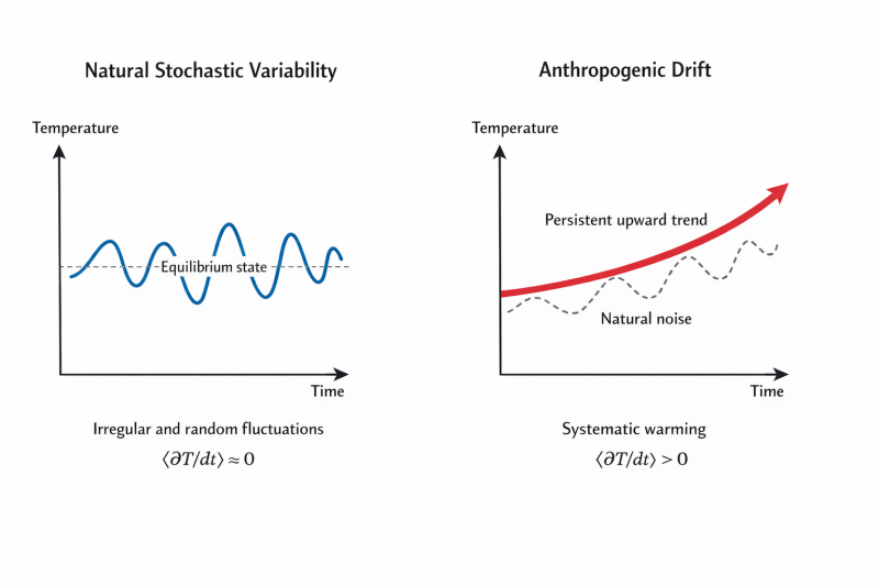
When natural climate variability is represented realistically as nonlinear and stochastic processes, their key property remains: they oscillate around an equilibrium state without a persistent unidirectional trend. Mathematically, this means that the long-term expectation value of the temperature time derivative is approximately zero unless external forcing changes systematically.
Adding anthropogenic forcing fundamentally alters the structure of the equation. A positive drift term appears in the system, which does not cancel out in the average of oscillations. This distinguishes current climate change from natural variability not merely by amplitude, but above all by the rate of change and the persistent imbalance in the energy budget.
In other words: although the climate system is chaotic and variable, its dynamics without sustained external forcing do not produce a continuous, accelerating warming trend. It is precisely this structural mathematical difference that defines the exceptional nature of the present situation.
(See the basic graphs)
Luo oma verkkosivustosi palvelussa Webador